Let’s walk through how to build a CNN from scratch using TensorFlow and Keras to classify images from the CIFAR-10 dataset. CIFAR-10 is a dataset containing 60,000 color images (32x32 pixels) across 10 classes.
import tensorflow as tf
from tensorflow.keras import layers, models
from tensorflow.keras.datasets import cifar10
from tensorflow.keras.utils import to_categorical
TensorFlow has it built-in:
(train_images, train_labels), (test_images, test_labels) = cifar10.load_data()
The images are stored as NumPy arrays, and the labels range from 0 to 9, corresponding to different categories like airplanes, cats, and trucks.
Preprocess
Neural networks perform best when input data is normalized. Since pixel values range from 0 to 255, we scale them down to [0,1]. We also convert the labels into categorical format:
# Normalize the images to the range [0, 1]
train_images = train_images.astype('float32') / 255
test_images = test_images.astype('float32') / 255

# One-hot encode the labels
train_labels = to_categorical(train_labels, 10)
test_labels = to_categorical(test_labels, 10)
Downloading data from https://www.cs.toronto.edu/~kriz/cifar-10-python.tar.gz
[1m170498071/170498071[0m [32m━━━━━━━━━━━━━━━━━━━━[0m[37m[0m [1m4s[0m 0us/step
print(f"Training samples: {train_images.shape[0]}")
print(f"Test samples: {test_images.shape[0]}")

print(f"Image shape: {train_images[0].shape}")  # Should be (32, 32, 3) (32x32 pixels, 3 channels)
print(f"Label: {train_labels[0]}")
Training samples: 50000
Test samples: 10000
Image shape: (32, 32, 3)
Label: [0. 0. 0. 0. 0. 0. 1. 0. 0. 0.]
Build the CNN model
Now, let’s architect our CNN. The idea is simple:
- Convolutional layers to extract features
- Pooling layers to downsample
- Dense layers to classify
from tensorflow.keras import layers, models
from tensorflow.keras.layers import Input

model = models.Sequential([
    Input(shape=(32, 32, 3)),
    layers.Conv2D(32, (3, 3), activation='relu', padding='same'),
    layers.BatchNormalization(),
    layers.Conv2D(32, (3, 3), activation='relu', padding='same'),
    layers.BatchNormalization(),
    layers.MaxPooling2D((2, 2)),
    layers.Dropout(0.2),

    layers.Conv2D(64, (3, 3), activation='relu', padding='same'),
    layers.BatchNormalization(),
    layers.Conv2D(64, (3, 3), activation='relu', padding='same'),
    layers.BatchNormalization(),
    layers.MaxPooling2D((2, 2)),
    layers.Dropout(0.3),

    layers.Conv2D(128, (3, 3), activation='relu', padding='same'),
    layers.BatchNormalization(),
    layers.Conv2D(128, (3, 3), activation='relu', padding='same'),
    layers.BatchNormalization(),
    layers.MaxPooling2D((2, 2)),
    layers.Dropout(0.4),

    layers.Flatten(),
    layers.Dense(256, activation='relu'),
    layers.BatchNormalization(),
    layers.Dropout(0.5),
    layers.Dense(10, activation='softmax')
])
Breaking it Down:
- First Conv Layer: 32 filters, 3x3 kernel, ReLU activation, and input shape of (32,32,3)
- MaxPooling Layer: Reduces spatial size, preventing overfitting
- Repeat: Increase filter size progressively (64 → 128)
- Flatten: Turns the feature map into a 1D vector
- Dense Layers: Fully connected layers for classification
- Softmax Output: Gives probability distribution over 10 classes
Data Augmentation
To improve generalization, let’s apply some random transformations to the training images:
from tensorflow.keras.preprocessing.image import ImageDataGenerator
datagen = ImageDataGenerator(
    width_shift_range=0.1,
    height_shift_range=0.1,
    horizontal_flip=True,
    rotation_range=15,
    zoom_range=0.1,
    fill_mode='nearest'
)

datagen.fit(train_images)
Compile and train
from tensorflow.keras.callbacks import EarlyStopping, ReduceLROnPlateau

# Callbacks
early_stopping = EarlyStopping(monitor='val_loss', patience=10, restore_best_weights=True)
reduce_lr = ReduceLROnPlateau(monitor='val_loss', factor=0.2, patience=5, min_lr=1e-04)
optimizer = tf.keras.optimizers.Adam(learning_rate=0.001)
model.compile(optimizer=optimizer, loss='categorical_crossentropy', metrics=['accuracy'])
history_2 = model.fit(datagen.flow(train_images, train_labels, batch_size=128),
          epochs=100,
          validation_data=(test_images, test_labels),
          callbacks=[early_stopping, reduce_lr])
Epoch 1/100
/usr/local/lib/python3.11/dist-packages/keras/src/trainers/data_adapters/py_dataset_adapter.py:121: UserWarning: Your `PyDataset` class should call `super().__init__(**kwargs)` in its constructor. `**kwargs` can include `workers`, `use_multiprocessing`, `max_queue_size`. Do not pass these arguments to `fit()`, as they will be ignored.
self._warn_if_super_not_called()
[1m391/391[0m [32m━━━━━━━━━━━━━━━━━━━━[0m[37m[0m [1m57s[0m 110ms/step - accuracy: 0.3175 - loss: 2.1918 - val_accuracy: 0.2486 - val_loss: 2.5132 - learning_rate: 0.0010
Epoch 2/100
[1m391/391[0m [32m━━━━━━━━━━━━━━━━━━━━[0m[37m[0m [1m29s[0m 75ms/step - accuracy: 0.5112 - loss: 1.3688 - val_accuracy: 0.6072 - val_loss: 1.0945 - learning_rate: 0.0010
Epoch 3/100
[1m391/391[0m [32m━━━━━━━━━━━━━━━━━━━━[0m[37m[0m [1m29s[0m 74ms/step - accuracy: 0.5946 - loss: 1.1477 - val_accuracy: 0.5630 - val_loss: 1.4816 - learning_rate: 0.0010
Epoch 4/100
[1m391/391[0m [32m━━━━━━━━━━━━━━━━━━━━[0m[37m[0m [1m40s[0m 72ms/step - accuracy: 0.6409 - loss: 1.0067 - val_accuracy: 0.6870 - val_loss: 0.9069 - learning_rate: 0.0010
Epoch 5/100
[1m391/391[0m [32m━━━━━━━━━━━━━━━━━━━━[0m[37m[0m [1m28s[0m 72ms/step - accuracy: 0.6765 - loss: 0.9170 - val_accuracy: 0.7003 - val_loss: 0.8689 - learning_rate: 0.0010
Epoch 6/100
[1m391/391[0m [32m━━━━━━━━━━━━━━━━━━━━[0m[37m[0m [1m31s[0m 79ms/step - accuracy: 0.7021 - loss: 0.8467 - val_accuracy: 0.7506 - val_loss: 0.7191 - learning_rate: 0.0010
Epoch 7/100
[1m391/391[0m [32m━━━━━━━━━━━━━━━━━━━━[0m[37m[0m [1m28s[0m 73ms/step - accuracy: 0.7209 - loss: 0.8030 - val_accuracy: 0.7133 - val_loss: 0.8441 - learning_rate: 0.0010
Epoch 8/100
[1m391/391[0m [32m━━━━━━━━━━━━━━━━━━━━[0m[37m[0m [1m29s[0m 74ms/step - accuracy: 0.7284 - loss: 0.7695 - val_accuracy: 0.7692 - val_loss: 0.6790 - learning_rate: 0.0010
Epoch 9/100
[1m391/391[0m [32m━━━━━━━━━━━━━━━━━━━━[0m[37m[0m [1m29s[0m 74ms/step - accuracy: 0.7452 - loss: 0.7343 - val_accuracy: 0.7563 - val_loss: 0.7184 - learning_rate: 0.0010
Epoch 10/100
[1m391/391[0m [32m━━━━━━━━━━━━━━━━━━━━[0m[37m[0m [1m28s[0m 73ms/step - accuracy: 0.7586 - loss: 0.7030 - val_accuracy: 0.7608 - val_loss: 0.7153 - learning_rate: 0.0010
Epoch 11/100
[1m391/391[0m [32m━━━━━━━━━━━━━━━━━━━━[0m[37m[0m [1m42s[0m 75ms/step - accuracy: 0.7663 - loss: 0.6796 - val_accuracy: 0.7632 - val_loss: 0.7433 - learning_rate: 0.0010
Epoch 12/100
[1m391/391[0m [32m━━━━━━━━━━━━━━━━━━━━[0m[37m[0m [1m29s[0m 73ms/step - accuracy: 0.7734 - loss: 0.6537 - val_accuracy: 0.7750 - val_loss: 0.6597 - learning_rate: 0.0010
Epoch 13/100
[1m391/391[0m [32m━━━━━━━━━━━━━━━━━━━━[0m[37m[0m [1m28s[0m 72ms/step - accuracy: 0.7802 - loss: 0.6382 - val_accuracy: 0.7962 - val_loss: 0.6104 - learning_rate: 0.0010
Epoch 14/100
[1m391/391[0m [32m━━━━━━━━━━━━━━━━━━━━[0m[37m[0m [1m41s[0m 72ms/step - accuracy: 0.7904 - loss: 0.6160 - val_accuracy: 0.7867 - val_loss: 0.6579 - learning_rate: 0.0010
Epoch 15/100
[1m391/391[0m [32m━━━━━━━━━━━━━━━━━━━━[0m[37m[0m [1m28s[0m 73ms/step - accuracy: 0.7939 - loss: 0.6026 - val_accuracy: 0.8176 - val_loss: 0.5443 - learning_rate: 0.0010
Epoch 16/100
[1m391/391[0m [32m━━━━━━━━━━━━━━━━━━━━[0m[37m[0m [1m29s[0m 75ms/step - accuracy: 0.7986 - loss: 0.5862 - val_accuracy: 0.8143 - val_loss: 0.5561 - learning_rate: 0.0010
Epoch 17/100
[1m391/391[0m [32m━━━━━━━━━━━━━━━━━━━━[0m[37m[0m [1m28s[0m 72ms/step - accuracy: 0.8044 - loss: 0.5669 - val_accuracy: 0.7965 - val_loss: 0.6193 - learning_rate: 0.0010
Epoch 18/100
[1m391/391[0m [32m━━━━━━━━━━━━━━━━━━━━[0m[37m[0m [1m28s[0m 72ms/step - accuracy: 0.8104 - loss: 0.5542 - val_accuracy: 0.8137 - val_loss: 0.5530 - learning_rate: 0.0010
Epoch 19/100
[1m391/391[0m [32m━━━━━━━━━━━━━━━━━━━━[0m[37m[0m [1m29s[0m 75ms/step - accuracy: 0.8077 - loss: 0.5544 - val_accuracy: 0.8201 - val_loss: 0.5278 - learning_rate: 0.0010
Epoch 20/100
[1m391/391[0m [32m━━━━━━━━━━━━━━━━━━━━[0m[37m[0m [1m29s[0m 74ms/step - accuracy: 0.8082 - loss: 0.5553 - val_accuracy: 0.7874 - val_loss: 0.6586 - learning_rate: 0.0010
Epoch 21/100
[1m391/391[0m [32m━━━━━━━━━━━━━━━━━━━━[0m[37m[0m [1m28s[0m 72ms/step - accuracy: 0.8144 - loss: 0.5402 - val_accuracy: 0.8222 - val_loss: 0.5407 - learning_rate: 0.0010
Epoch 22/100
[1m391/391[0m [32m━━━━━━━━━━━━━━━━━━━━[0m[37m[0m [1m41s[0m 73ms/step - accuracy: 0.8178 - loss: 0.5192 - val_accuracy: 0.8068 - val_loss: 0.5975 - learning_rate: 0.0010
Epoch 23/100
[1m391/391[0m [32m━━━━━━━━━━━━━━━━━━━━[0m[37m[0m [1m30s[0m 77ms/step - accuracy: 0.8191 - loss: 0.5222 - val_accuracy: 0.8403 - val_loss: 0.4870 - learning_rate: 0.0010
Epoch 24/100
[1m391/391[0m [32m━━━━━━━━━━━━━━━━━━━━[0m[37m[0m [1m31s[0m 78ms/step - accuracy: 0.8234 - loss: 0.5109 - val_accuracy: 0.8436 - val_loss: 0.4622 - learning_rate: 0.0010
Epoch 25/100
[1m391/391[0m [32m━━━━━━━━━━━━━━━━━━━━[0m[37m[0m [1m29s[0m 74ms/step - accuracy: 0.8249 - loss: 0.5052 - val_accuracy: 0.8352 - val_loss: 0.4972 - learning_rate: 0.0010
Epoch 26/100
[1m391/391[0m [32m━━━━━━━━━━━━━━━━━━━━[0m[37m[0m [1m41s[0m 75ms/step - accuracy: 0.8270 - loss: 0.4999 - val_accuracy: 0.8437 - val_loss: 0.4592 - learning_rate: 0.0010
Epoch 27/100
[1m391/391[0m [32m━━━━━━━━━━━━━━━━━━━━[0m[37m[0m [1m29s[0m 75ms/step - accuracy: 0.8307 - loss: 0.4923 - val_accuracy: 0.8508 - val_loss: 0.4435 - learning_rate: 0.0010
Epoch 28/100
[1m391/391[0m [32m━━━━━━━━━━━━━━━━━━━━[0m[37m[0m [1m30s[0m 77ms/step - accuracy: 0.8351 - loss: 0.4802 - val_accuracy: 0.8163 - val_loss: 0.5592 - learning_rate: 0.0010
Epoch 29/100
[1m391/391[0m [32m━━━━━━━━━━━━━━━━━━━━[0m[37m[0m [1m29s[0m 74ms/step - accuracy: 0.8325 - loss: 0.4802 - val_accuracy: 0.8377 - val_loss: 0.4978 - learning_rate: 0.0010
Epoch 30/100
[1m391/391[0m [32m━━━━━━━━━━━━━━━━━━━━[0m[37m[0m [1m29s[0m 74ms/step - accuracy: 0.8359 - loss: 0.4730 - val_accuracy: 0.8449 - val_loss: 0.4665 - learning_rate: 0.0010
Epoch 31/100
[1m391/391[0m [32m━━━━━━━━━━━━━━━━━━━━[0m[37m[0m [1m29s[0m 75ms/step - accuracy: 0.8378 - loss: 0.4694 - val_accuracy: 0.8378 - val_loss: 0.4860 - learning_rate: 0.0010
Epoch 32/100
[1m391/391[0m [32m━━━━━━━━━━━━━━━━━━━━[0m[37m[0m [1m28s[0m 73ms/step - accuracy: 0.8424 - loss: 0.4558 - val_accuracy: 0.8451 - val_loss: 0.4616 - learning_rate: 0.0010
Epoch 33/100
[1m391/391[0m [32m━━━━━━━━━━━━━━━━━━━━[0m[37m[0m [1m28s[0m 72ms/step - accuracy: 0.8508 - loss: 0.4329 - val_accuracy: 0.8677 - val_loss: 0.3939 - learning_rate: 2.0000e-04
Epoch 34/100
[1m391/391[0m [32m━━━━━━━━━━━━━━━━━━━━[0m[37m[0m [1m29s[0m 75ms/step - accuracy: 0.8550 - loss: 0.4145 - val_accuracy: 0.8676 - val_loss: 0.4048 - learning_rate: 2.0000e-04
Epoch 35/100
[1m391/391[0m [32m━━━━━━━━━━━━━━━━━━━━[0m[37m[0m [1m31s[0m 78ms/step - accuracy: 0.8600 - loss: 0.4079 - val_accuracy: 0.8739 - val_loss: 0.3824 - learning_rate: 2.0000e-04
Epoch 36/100
[1m391/391[0m [32m━━━━━━━━━━━━━━━━━━━━[0m[37m[0m [1m33s[0m 84ms/step - accuracy: 0.8654 - loss: 0.3936 - val_accuracy: 0.8750 - val_loss: 0.3796 - learning_rate: 2.0000e-04
Epoch 37/100
[1m391/391[0m [32m━━━━━━━━━━━━━━━━━━━━[0m[37m[0m [1m31s[0m 80ms/step - accuracy: 0.8649 - loss: 0.3967 - val_accuracy: 0.8711 - val_loss: 0.3834 - learning_rate: 2.0000e-04
Epoch 38/100
[1m391/391[0m [32m━━━━━━━━━━━━━━━━━━━━[0m[37m[0m [1m32s[0m 83ms/step - accuracy: 0.8656 - loss: 0.3891 - val_accuracy: 0.8717 - val_loss: 0.3969 - learning_rate: 2.0000e-04
Epoch 39/100
[1m391/391[0m [32m━━━━━━━━━━━━━━━━━━━━[0m[37m[0m [1m32s[0m 81ms/step - accuracy: 0.8656 - loss: 0.3887 - val_accuracy: 0.8764 - val_loss: 0.3759 - learning_rate: 2.0000e-04
Epoch 40/100
[1m391/391[0m [32m━━━━━━━━━━━━━━━━━━━━[0m[37m[0m [1m30s[0m 77ms/step - accuracy: 0.8680 - loss: 0.3839 - val_accuracy: 0.8770 - val_loss: 0.3748 - learning_rate: 2.0000e-04
Epoch 41/100
[1m391/391[0m [32m━━━━━━━━━━━━━━━━━━━━[0m[37m[0m [1m31s[0m 80ms/step - accuracy: 0.8660 - loss: 0.3862 - val_accuracy: 0.8744 - val_loss: 0.3792 - learning_rate: 2.0000e-04
Epoch 42/100
[1m391/391[0m [32m━━━━━━━━━━━━━━━━━━━━[0m[37m[0m [1m30s[0m 76ms/step - accuracy: 0.8717 - loss: 0.3765 - val_accuracy: 0.8770 - val_loss: 0.3684 - learning_rate: 2.0000e-04
Epoch 43/100
[1m391/391[0m [32m━━━━━━━━━━━━━━━━━━━━[0m[37m[0m [1m31s[0m 80ms/step - accuracy: 0.8678 - loss: 0.3841 - val_accuracy: 0.8774 - val_loss: 0.3687 - learning_rate: 2.0000e-04
Epoch 44/100
[1m391/391[0m [32m━━━━━━━━━━━━━━━━━━━━[0m[37m[0m [1m30s[0m 76ms/step - accuracy: 0.8696 - loss: 0.3745 - val_accuracy: 0.8770 - val_loss: 0.3686 - learning_rate: 2.0000e-04
Epoch 45/100
[1m391/391[0m [32m━━━━━━━━━━━━━━━━━━━━[0m[37m[0m [1m29s[0m 74ms/step - accuracy: 0.8687 - loss: 0.3792 - val_accuracy: 0.8724 - val_loss: 0.3866 - learning_rate: 2.0000e-04
Epoch 46/100
[1m391/391[0m [32m━━━━━━━━━━━━━━━━━━━━[0m[37m[0m [1m30s[0m 75ms/step - accuracy: 0.8690 - loss: 0.3730 - val_accuracy: 0.8729 - val_loss: 0.3892 - learning_rate: 2.0000e-04
Epoch 47/100
[1m391/391[0m [32m━━━━━━━━━━━━━━━━━━━━[0m[37m[0m [1m29s[0m 75ms/step - accuracy: 0.8707 - loss: 0.3763 - val_accuracy: 0.8837 - val_loss: 0.3567 - learning_rate: 2.0000e-04
Epoch 48/100
[1m391/391[0m [32m━━━━━━━━━━━━━━━━━━━━[0m[37m[0m [1m30s[0m 76ms/step - accuracy: 0.8703 - loss: 0.3798 - val_accuracy: 0.8774 - val_loss: 0.3767 - learning_rate: 2.0000e-04
Epoch 49/100
[1m391/391[0m [32m━━━━━━━━━━━━━━━━━━━━[0m[37m[0m [1m29s[0m 74ms/step - accuracy: 0.8730 - loss: 0.3633 - val_accuracy: 0.8797 - val_loss: 0.3708 - learning_rate: 2.0000e-04
Epoch 50/100
[1m391/391[0m [32m━━━━━━━━━━━━━━━━━━━━[0m[37m[0m [1m29s[0m 74ms/step - accuracy: 0.8713 - loss: 0.3687 - val_accuracy: 0.8732 - val_loss: 0.3910 - learning_rate: 2.0000e-04
Epoch 51/100
[1m391/391[0m [32m━━━━━━━━━━━━━━━━━━━━[0m[37m[0m [1m33s[0m 84ms/step - accuracy: 0.8692 - loss: 0.3750 - val_accuracy: 0.8772 - val_loss: 0.3709 - learning_rate: 2.0000e-04
Epoch 52/100
[1m391/391[0m [32m━━━━━━━━━━━━━━━━━━━━[0m[37m[0m [1m31s[0m 78ms/step - accuracy: 0.8725 - loss: 0.3645 - val_accuracy: 0.8752 - val_loss: 0.3774 - learning_rate: 2.0000e-04
Epoch 53/100
[1m391/391[0m [32m━━━━━━━━━━━━━━━━━━━━[0m[37m[0m [1m28s[0m 73ms/step - accuracy: 0.8794 - loss: 0.3517 - val_accuracy: 0.8867 - val_loss: 0.3440 - learning_rate: 1.0000e-04
Epoch 54/100
[1m391/391[0m [32m━━━━━━━━━━━━━━━━━━━━[0m[37m[0m [1m29s[0m 73ms/step - accuracy: 0.8740 - loss: 0.3640 - val_accuracy: 0.8806 - val_loss: 0.3628 - learning_rate: 1.0000e-04
Epoch 55/100
[1m391/391[0m [32m━━━━━━━━━━━━━━━━━━━━[0m[37m[0m [1m30s[0m 76ms/step - accuracy: 0.8778 - loss: 0.3567 - val_accuracy: 0.8825 - val_loss: 0.3566 - learning_rate: 1.0000e-04
Epoch 56/100
[1m391/391[0m [32m━━━━━━━━━━━━━━━━━━━━[0m[37m[0m [1m29s[0m 73ms/step - accuracy: 0.8769 - loss: 0.3597 - val_accuracy: 0.8810 - val_loss: 0.3614 - learning_rate: 1.0000e-04
Epoch 57/100
[1m391/391[0m [32m━━━━━━━━━━━━━━━━━━━━[0m[37m[0m [1m29s[0m 74ms/step - accuracy: 0.8741 - loss: 0.3616 - val_accuracy: 0.8805 - val_loss: 0.3596 - learning_rate: 1.0000e-04
Epoch 58/100
[1m391/391[0m [32m━━━━━━━━━━━━━━━━━━━━[0m[37m[0m [1m42s[0m 75ms/step - accuracy: 0.8779 - loss: 0.3498 - val_accuracy: 0.8795 - val_loss: 0.3647 - learning_rate: 1.0000e-04
Epoch 59/100
[1m391/391[0m [32m━━━━━━━━━━━━━━━━━━━━[0m[37m[0m [1m29s[0m 75ms/step - accuracy: 0.8795 - loss: 0.3512 - val_accuracy: 0.8799 - val_loss: 0.3647 - learning_rate: 1.0000e-04
Epoch 60/100
[1m391/391[0m [32m━━━━━━━━━━━━━━━━━━━━[0m[37m[0m [1m42s[0m 77ms/step - accuracy: 0.8792 - loss: 0.3554 - val_accuracy: 0.8840 - val_loss: 0.3538 - learning_rate: 1.0000e-04
Epoch 61/100
[1m391/391[0m [32m━━━━━━━━━━━━━━━━━━━━[0m[37m[0m [1m29s[0m 74ms/step - accuracy: 0.8782 - loss: 0.3521 - val_accuracy: 0.8799 - val_loss: 0.3659 - learning_rate: 1.0000e-04
Epoch 62/100
[1m391/391[0m [32m━━━━━━━━━━━━━━━━━━━━[0m[37m[0m [1m29s[0m 75ms/step - accuracy: 0.8830 - loss: 0.3409 - val_accuracy: 0.8852 - val_loss: 0.3462 - learning_rate: 1.0000e-04
Epoch 63/100
[1m391/391[0m [32m━━━━━━━━━━━━━━━━━━━━[0m[37m[0m [1m29s[0m 74ms/step - accuracy: 0.8780 - loss: 0.3476 - val_accuracy: 0.8830 - val_loss: 0.3530 - learning_rate: 1.0000e-04
Evaluation
test_loss, test_acc = model.evaluate(test_images, test_labels)
print(f"Test accuracy: {test_acc}")
[1m313/313[0m [32m━━━━━━━━━━━━━━━━━━━━[0m[37m[0m [1m1s[0m 3ms/step - accuracy: 0.8892 - loss: 0.3440
Test accuracy: 0.8866999745368958
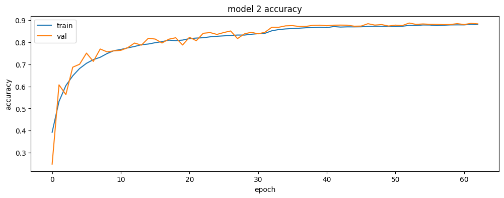
Not bad for a simple CNN! We can improve the performance later on by tweaking hyperparameters or using more complex architectures.
# summarize history for accuracy
import matplotlib.pyplot as plt
plt.figure(figsize=(12, 4))
plt.plot(history_2.history['accuracy'])
plt.plot(history_2.history['val_accuracy'])
plt.title('model 2 accuracy')
plt.ylabel('accuracy')
plt.xlabel('epoch')
plt.legend(['train', 'val'], loc='upper left')
plt.show()
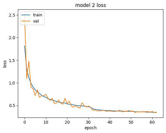
# summarize history for loss
plt.plot(history_2.history['loss'])
plt.plot(history_2.history['val_loss'])
plt.title('model 2 loss')
plt.ylabel('loss')
plt.xlabel('epoch')
plt.legend(['train', 'val'], loc='upper left')
plt.show()
Prediction
Since we saved the model, let’s trying loading the saved model and predict with a new image.
from tensorflow.keras.preprocessing import image
import numpy as np
import matplotlib.pyplot as plt
from google.colab import drive

drive.mount('/content/drive')

# Load the saved model
loaded_model = tf.keras.models.load_model('/content/drive/MyDrive/my_cifar10_model.keras')

# Load and preprocess the single image
image_path = '/content/drive/MyDrive/bird_sample1.jpg'
img = image.load_img(image_path, target_size=(32, 32))
img_array = image.img_to_array(img)
img_array = np.expand_dims(img_array, axis=0)
img_array = img_array / 255.0

prediction = loaded_model.predict(img_array)
predicted_class = np.argmax(prediction, axis=1)[0]

# CIFAR-10 class labels (in order)
class_labels = ['airplane', 'automobile', 'bird', 'cat', 'deer', 'dog', 'frog', 'horse', 'ship', 'truck']

# Get the predicted class label
predicted_label = class_labels[predicted_class]

# Visualize the image and prediction
plt.imshow(image.load_img(image_path))
plt.title(f"Predicted: {predicted_label}")
plt.axis('off')  # Turn off axis labels
plt.show()

print(f"Predicted class index: {predicted_class}")
print(f"Predicted class label: {predicted_label}")
Drive already mounted at /content/drive; to attempt to forcibly remount, call drive.mount("/content/drive", force_remount=True).
[1m1/1[0m [32m━━━━━━━━━━━━━━━━━━━━[0m[37m[0m [1m1s[0m 1s/step
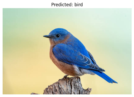
Predicted class index: 2
Predicted class label: bird
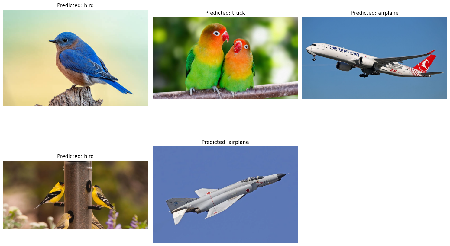
Now let’s download a couple of pictures from Google and test out the model.
import os

image_dir = '/content/drive/MyDrive/test_samples_cifar/'

# Function to load, preprocess, and predict a single image
def predict_image(image_path):
    img = image.load_img(image_path, target_size=(32, 32))
    img_array = image.img_to_array(img)
    img_array = np.expand_dims(img_array, axis=0)
    img_array = img_array / 255.0
    prediction = loaded_model.predict(img_array)
    predicted_class = np.argmax(prediction, axis=1)[0]
    return predicted_class

# Process all images in a folder
image_files = [f for f in os.listdir(image_dir) if f.endswith(('.jpg', '.jpeg', '.png', 'webp'))]

plt.figure(figsize=(15, 5 * (len(image_files) // 3 + 1)))  # Adjust figure size

for i, image_file in enumerate(image_files):
    image_path = os.path.join(image_dir, image_file)
    predicted_class = predict_image(image_path)
    predicted_label = class_labels[predicted_class]

    plt.subplot(len(image_files) // 3 + 1, 3, i + 1)
    plt.imshow(image.load_img(image_path))
    plt.title(f"Predicted: {predicted_label}")
    plt.axis('off')

plt.tight_layout()  # Improve spacing
plt.show()

# Print predictions for each image
for image_file in image_files:
    image_path = os.path.join(image_dir, image_file)
    predicted_class = predict_image(image_path)
    predicted_label = class_labels[predicted_class]
    print(f"Image: {image_file}, Predicted: {predicted_label} (Class Index: {predicted_class})")
[1m1/1[0m [32m━━━━━━━━━━━━━━━━━━━━[0m[37m[0m [1m0s[0m 75ms/step
Image: bird_sample1.jpg, Predicted: bird (Class Index: 2)
[1m1/1[0m [32m━━━━━━━━━━━━━━━━━━━━[0m[37m[0m [1m0s[0m 51ms/step
Image: bird_sample2.jpg, Predicted: truck (Class Index: 9)
[1m1/1[0m [32m━━━━━━━━━━━━━━━━━━━━[0m[37m[0m [1m0s[0m 52ms/step
Image: airplane_sample2.jpg, Predicted: airplane (Class Index: 0)
[1m1/1[0m [32m━━━━━━━━━━━━━━━━━━━━[0m[37m[0m [1m0s[0m 50ms/step
Image: bird_sample3.webp, Predicted: bird (Class Index: 2)
[1m1/1[0m [32m━━━━━━━━━━━━━━━━━━━━[0m[37m[0m [1m0s[0m 49ms/step
Image: airplane_sample1.webp, Predicted: airplane (Class Index: 0)
Oops. It seems to classify the second picture as a truck… Poor parrots. But you get the idea. Let’s do it again another time.